Chapter 4 Property Stolen and Recovered (Supplement to Return A)

The Property Stolen and Recovered dataset, also known as the Supplement to Return A³⁴, tracks monthly data on property crimes (theft, burglary, robbery, and motor vehicle theft), with information on where the crime occurred, what was stolen, and the estimated value of the stolen property. The “recovered” part of this dataset covers the type and value of property recovered. Like most other SRS datasets this is at the agency-month level so you can, for example, learn how often burglaries occur at the victim’s home during the day, and if that rate changes over the year or differs across agencies. The data, however, provides no information about the offender or the victim (other than if the victim was an individual or a commercial business ³⁵).

The value of stolen property is generally based on the victim’s estimate. However, police are supposed to use the market value for items, even if that value is different than the victim’s estimate. Because of this, the reported values should be treated as rough estimates. And since this is the victim’s reporting it may be incomplete. For example, say a person was burglarized and had 10 of their possessions stolen but they only realized that nine items were taken. They would report these nine items to the police but the tenth item would be left out of our data.

This dataset provides a rough estimate of the cost of crime, limited to the value of stolen property. It excludes other important costs such as physical injuries, emotional harm, or preventative expenses (e.g., home security systems). For some types of stolen property we also know the number of offenses that occurred meaning that we can use both of these numbers to create an average value of stolen property per offense. An issue here is that we only have the monthly number of offenses and monthly value of the property. We can make the average value per offense but will not know if our average is affected by having an outlier in the data - such as one theft of an extremely expensive item.

Before getting into the details of this data, let us look at one example of how this data can measure property crime in a few different ways, and look at common pitfalls. We will look at home burglaries that occur during the day in Philadelphia. Figure 4.1 shows the annual number of daytime home burglaries Philadelphia and in recent years it has declined sharply into having the fewest on record in 2020 followed by a very low number of crimes in 2021 and 2022. So citywide, Philadelphia has never been safer (averaging across the last few years) when it comes to the number of daytime home burglaries. As you should be aware by this point in the book, SRS data is optional and not all agencies report data every year.

In this case, 2019-2021 data are all partial-year reports, with only 9, 4, and 9 months, respectively, reported for these years. Every previous year other than 1974, 1975, 1988, and 1989³⁶ had a full 12-months of data reported. So it makes sense the 2019-2021 had fewer crimes if they only submitted data for part of the year. This is something that is pretty obvious - you cannot compare 12 months of data with <12 months of data - but it is a common mistake so you should check how many months are reported every time you compare multiple years.

Figure 4.1: The annual number of daytime home burglaries reported in Philadelphia, PA, 1960-2023.

When considering the cost of crime, we also want to know the actually monetary cost of that incident. Figure 4.2 measures this cost of crime by showing the annual value of the property stolen for daytime home burglaries in Philadelphia. The years without 12 months of data are excluded from the figure. Like many variables in this dataset, there is no reported crime value until 1964, so the data shows a value of 0 from 1960-1963.

The trend here is different than the previous graph which showed movement in the number of burglaries but not major trend changes until the 2010s; here is a steady increase over the long term, though with varying speed of increase, until it peaked in the late 2000s/early 2010s before declining substantially in recent years. While the number of burglaries peaked in the early 1980s, the total value of burglaries did not peak until the early 2010s, so the cost of this crime (even this very narrow measure of cost) cannot be ascertained from knowing the number of burglaries alone. From this measure we can say that daytime home burglaries were worse in the early 2010s and are substantially better currently.

Figure 4.2: The total annual cost of daytime home burglaries in Philadelphia.

The final way we can measure daytime home burglaries is to put the previous variables together to look at the cost per burglary. This will give us the average amount of property stolen from each burglary victim. Figure 4.3 shows the average cost per burglary for each year of data available. Now we have a different story than the other graphs. Even though the number of daytime home burglaries declined substantially over the last decade and the total cost is around the level seen in the 1980s, the cost per burglary remains high in recent years, though down from the peak in the mid-2010s. This suggests that while burglaries are down, the burden on each burglary victim has continued to grow.

A perhaps obvious issue here is that we have no way to determining how much outliers are affecting results. If one year has, for example, a home burglary where $10 million worth of jewelry is stolen then that year’s total value of property stolen would be much higher just due to a single burglary. There is, unfortunately, no way to handle this in this dataset, though NIBRS has similar data which does allow you to check for outliers.³⁷

Figure 4.3: The annual cost per burglary for daytime home burglaries in Philadelphia, 1960-2023.

Part of this - and part of the long-term increase seen in Figure 4.2 - is simply due to inflation. A dollar in 1964, the first year we have data on the value of burglaries, is worth $9.84 in 2023, according to the Bureau of Labor Statistics.³⁸ The values in this data are not adjusted for inflation so you need to do that adjustment yourself before any analyses, otherwise your results will be quite a bit off. When we adjust all values to 2023 dollars, as shown in Figure ??, the trend becomes changes a bit. There’s still a steady increase in cost per burglary over time but it is far more gradual than in Figure 4.3. And now the difference from the cost in early years and late years are far smaller.

4.1 Agencies reporting

The data is available from 1960 to the present, though olders years of data have fewer variables reported. Figure 4.4 show the number of agencies each year that reported at least one month during that year. In the first several years of data barely any agencies reported data and then it spiked around 1966 to over 6,000 agencies per year then grew quickly until over 12,000 agencies reported data in the late 1970s. From here it actually gradually declined until fewer than 12,000 agencies in the late 1990s before reversing course again and growing to about 15,000 agencies by 2019 - down several hundred agencies from the peak a few years earlier. We see the now-typical drop in 2021 as a result of the FBI’s death of SRS and then the partial recovery in 2022 when SRS was reborn. The agencies that still reported in 2021 did so by reporting NIBRS data which the FBI converted to this format.

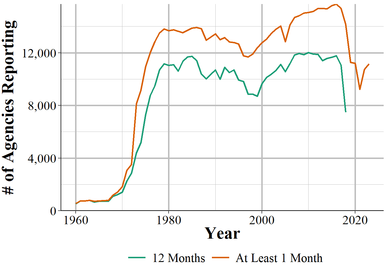
Figure 4.4: The annual number of police agencies that report at least month of data and 12 months of data that year.

Since this data is called the “Supplement to Return A” we would expect that the agencies that report here are the same as the ones that report to the Offenses Known and Clearances by Arrest data, which is also called the Return A dataset. Figure 4.5 shows the percent of agencies in this dataset that are report at least one month of Return A data. Except for the first several years of data in the 1960s, we can see that most years have nearly all agencies reporting to both, though this has declined slightly in recent years. Since the late 1970s, over 90% of agencies that report to the Offenses Known data also report to this dataset.

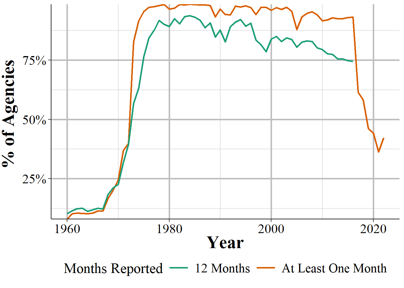
Figure 4.5: The percent of agencies in the Supplement to Return A data that report at least one month of data, and all 12 months of data, and are also in the Offenses Known and Clearances by Arrest (Return A) data in that year, 1960-2023.

When filtering the data to agencies that report a full 12 months of both the Return A and the Supplement to Return A, shown in Figure ??, trends are quite similar to Figure 4.5 though now the average percent is around 75% rather than 90%. This translates to around 11k agencies though it drops starting in 2018 until fewer than 8,500 agencies report full data to both datasets in 2022.

4.2 Important variables

This data can really be broken into two parts: the monthly number of property (as well as robbery) crimes that occur that are more detailed than in the Offenses Known data, and the value of the property stolen (and recovered) from these crimes. For each category I present the complete breakdown of the available offenses/items stolen and describe some of the important issues to know about them. Like other SRS data, there are also variables that provide information about the agency - ORI codes, population under jurisdiction - the month and year that the data covers, and how many months reported data.

4.2.1 A more detailed breakdown of property (and robbery) crimes

The first part of this data is just a monthly (or yearly if you aggregate the data) number of crimes of each type reported to the police and that a police investigation discovered actually happened.³⁹. There are six crimes and their subsets included here: burglary, theft, robbery, and motor vehicle theft. The remaining two are rape and murder, but they do not break down these crimes into any subcategories and are only available starting in 1974.

Though this data starts in 1960, not all variables are available then. 1963 and 1964 saw many new variables added - the values in these variables are reported as 0 in previous years - and in 1974 and 1975 even more variables were added. In 1963 the value of burglaries where the time of the burglary was known, thefts broken down into categories based on the value of property taken, thefts of car parts, theft from cars, shoplifting, and “other” thefts was added to the data. In the following year this data began including the value of property stolen from burglaries where the time of the burglary was unknown was added as well as thefts of bicycles, from “coin operated machines” (i.e. vending machines), purse snatching, and pick pocketing. The value of property stolen during rapes and murders was first reported in 1974. Finally, 1975 was the last year with new variables, with this year including consumable goods, stolen guns, household goods, livestock, office equipment and electronics, and sound and picture equipment.

The complete list of each subsection and a brief definition for the non-obvious ones are presented below.

• Burglary
  • Home/residence during the day (6AM - 5:59PM)
  • Home/residence during the night (6PM - 5:59AM)
  • Home residence at unknown time
  • Non-residence (i.e. all buildings other than victim’s home) during the day (6:00AM - 5:59PM)
  • Non-residence (i.e. all buildings other than victim’s home) during the night (6:00PM - 5:59AM)
  • Non-residence (i.e. all buildings other than victim’s home) at unknown time
• Theft/larceny (excluding of a motor vehicle)
  • Less than $50
  • $50-$199
  • $200 and up
  • Pick pocket
  • Purse snatching
  • Shoplifting
  • Stealing from a car (but not stealing the car itself)
  • Stealing parts of a car, such as the car battery or the tires
  • Stealing a bicycle
  • Stealing from a building where the offender is allowed to be in (and is not counted already as shoplifting)
  • Stealing from a “coin operated machine” which is mainly vending machines
  • All other thefts
• Robbery
  • Highway - This is an old term to say a place is outside and in generally accessible and visible areas. This includes robberies on public streets and alleys.
  • Commercial building - This is robberies in a business other than ones stated below. Includes restaurants, stores, hotels, bars.
  • Gas station
  • Chain/convenience store - a neighborhood store that generally is open late and sells food
  • Home/residence
  • Bank
  • Miscellaneous/other - This is all other robberies not already covered.
• Motor vehicle theft
  • Stolen in current agency’s jurisdiction and found by that agency
  • Stolen in current agency’s jurisdiction and found by another agency
  • Stolen in another agency’s jurisdiction and recovered by current agency
• Murder
• Rape

Burglary is reported based on whether the building burgled was the victim’s residence or not, and also the time of the burglary. Time is either during the day (6AM-5:59PM) or night (6PM-5:59AM) or if the time is unknown. Data is available since 1960 for both the day and night burglaries, but only since 1964 for the unknown time burglaries. For robbery, the subcategories are based on where the robberies occurred such as if it happened in a bank, a gas station, or a street.

Theft is divided into two groups. The first group is based on the value of items stolen: less than $50, $50-$199, and $200 and up. The second group of thefts is broken into the type of theft such as a shoplifting or stealing from someone’s car. All theft variables begin in 1960 other than thefts from a coin machine and from a building which start in 1964 and the miscellaneous “All other thefts” variable that has data starting in 1961. Finally, motor vehicle theft is broken into where the stolen vehicle was stolen and found: stolen in the reporting agency’s jurisdiction and found by the same agency, stolen in the reporting agency’s jurisdiction and found by a different agency, and stolen in a different agency’s jurisdiction and found by the reporting agency.

The first group is a useful example of a problem in this data, which can be seen happening in 1974. In Figure 4.6 we use data from all agencies in the United States that reported 12 months of data to see the share of the total value of thefts by the three value categories. Thefts of between $50 and $200 start as the most common at nearly 60% of thefts in 1960 and steadily decline to under 20% by 2022. Thefts of over $200 increase steadily from about 28% of thefts in 1960 to almost 50% in 1973 and then drop to 16% in 1974. Then the share of thefts over $200 slowly increases over time to end our data at over 55% of thefts. Thefts valued at under $50 have a near mirror trend as over $200, starting at under 15% in 1960, declining a bit after that and then massively spiking to 49% in 1974 before starting a slow decline to 27% in 2022.

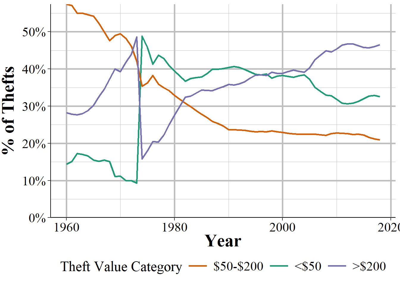
Figure 4.6: The annual breakdown in total theft value by the three value categories: less than $50, $50-$199, and $200 and over, among all agencies that reported 12 months of data in that year, 1960-2023.

What caused this weird swap of the less than $50 and at least $200 values? Well, part of it is that different agencies report over time so year-to-year comparisons are not really appropriate. Even agencies that report every year may report only some months of data. But we corrected that by filtering the data shown in Figure 4.6 to only agencies that reported 12 months of data. Unfortunately, even doing that is not sufficient, as we can see below.

Figure 4.7 replicates Figure 4.6 but now only for agencies in California and zooms in to 1960-1980. In every agency in California there were zero reported thefts under $50 starting in 1969 and ending in 1974. The number of thefts between $50 and $200, and thefts over $200 increased, suggesting that agencies still reported the data but in the wrong category. Then in 1974 the thefts under $50 were reported once again and the number of thefts in the other categories dropped. Given that the entire state changed reporting practices I believe that this was from either a policy at the state-level or some data error by the state before they sent the data to the FBI. It certainly is not true that there were zero thefts under $50 for five years in California.

Luckily in this case it was a fairly easy error to find - though I suspect that California is only part of the problem. But it reveals a broader issue with UCR data. The purpose of the data is that it is “Uniform,” but we see that entire states can stop reporting certain data even when they say that they report data for all 12 months. Since UCR data is voluntary, agencies can report some, all, or none of the data, which makes it frustrating and time-consuming for researchers to ensure that the results in the data are real and not simply caused by reporting issues.

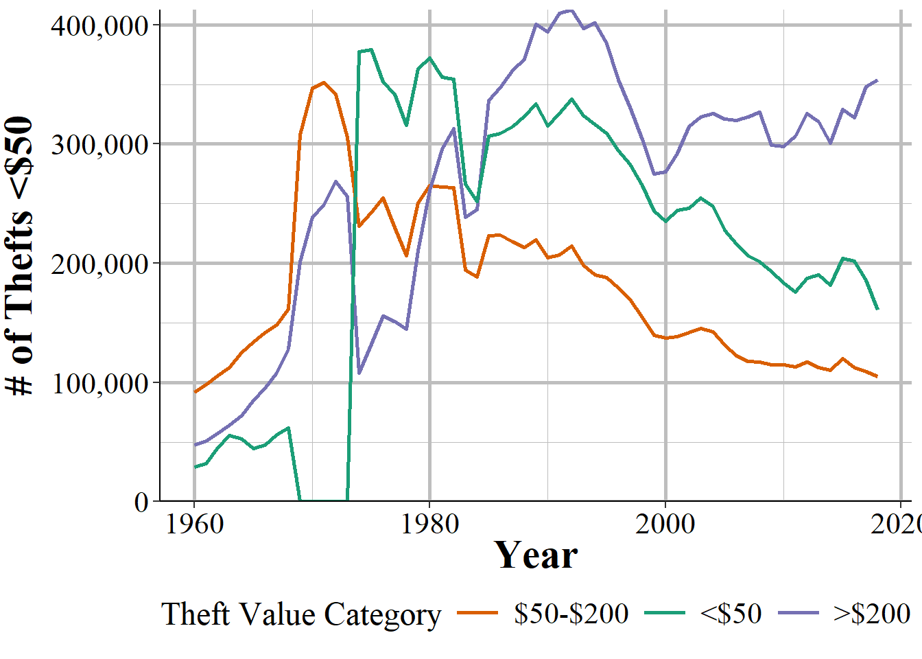
Figure 4.7: The annual breakdown in total theft value by the three value categories: less than $50, $50-$199, and $200 and over, among agencies in California that reported 12 months of data in that year, 1960-1980

4.2.2 The value of property stolen

The next set of variables is the value of the property stolen in each crime, as well as the value of property stolen broken down by the type of property (e.g. clothing, electronics, etc.). To be clear, this is only the value of the property stolen during the crime. The cost of any injuries (mental or physical) or any lasting cost to the victim, their family, and society for these crimes are not included. This, of course, vastly underestimates the cost of these crimes so please understand that while this is a measure of the cost of crime, it is only a narrow slice of the true cost.

The cost is the cost for the victim to replace the stolen item. So the current market price for that item (though factoring in the current state the item is in, e.g. if it is already damaged) and, for businesses, the cost to buy that item and not the cost they sell it for. While the police can ask the victim how much the property was worth, they are not required to use the exact amount given as victims may exaggerate the value of items. This is not an exact science, so I recommend only interpreting these values as estimates - and potentially rough estimates. None of this data is adjusted for inflation so if you are comparing values over time you will need to do that adjustment yourself.

The value of the property stolen is broken into two overlapping categories: by crime type, and by type of property that was stolen. These are the exact same categories as covered in Section 4.2.1 but now is the dollar amount of the items stolen from those types of crimes. The second group is what type of item, based on several discrete categories, was stolen. Please note that multiple items can be stolen in each category and this data counts the property stolen for each crime type as well as for each item type. So if you sum up all of the crime variables and all of the item type variables together you will over-count the value of property stolen. Each of the categories and their definitions are detailed below.

Some of these will overlap with the list in the previous section, though for completeness I will repeat them.

Here are the subsets of crimes:

• Burglary
  • Home/residence during the day (6:00am - 5:59pm)
  • Home/residence during the night (6:00pm - 5:59am)
  • Home residence at unknown time
  • Non-residence (i.e. all buildings other than victim’s home) during the day (6:00am - 5:59pm)
  • Non-residence (i.e. all buildings other than victim’s home) during the night (6:00pm - 5:59am)
  • Non-residence (i.e. all buildings other than victim’s home) at unknown time
• Theft/larceny (excluding of a motor vehicle)
  • Less than $50
  • $50-$199
  • $200 and up
  • Pick pocket
  • Purse snatching
  • Shoplifting
  • Stealing from a car (but not stealing the car itself)
  • Stealing parts of a car, such as the car battery or the tires
  • Stealing a bicycle
  • Stealing from a building where the offender is allowed to be in (and is not counted already as shoplifting)
  • Stealing from a “coin operated machine” which is mainly vending machines
  • All other thefts
• Robbery
  • Highway - This is an old term to say a place is outside and in generally accessible and visible areas. This includes robberies on public streets and alleys.
  • Commercial building - This is robberies in a business other than ones stated below. Includes restaurants, stores, hotels, bars.
  • Gas station
  • Chain/convenience store - a neighborhood store that generally is open late and sells food
  • Home/residence
  • Bank
  • Miscellaneous/other - This is all other robberies not already covered.
• Motor vehicle theft
  • Stolen in current agency’s jurisdiction and found by that agency
  • Stolen in current agency’s jurisdiction and found by another agency
  • Stolen in another agency’s jurisdiction and recovered by current agency
• Murder
• Rape

And here are the items stolen:

• Currency
  • This includes all money and signed documents that can be exchanged for money (e.g. checks). Blank checks and credit and debit cards are not included (they are in the Miscellaneous/other category)
• Jewelry and “precious metals”
  • Only metals that are considered high value are included here. Metals that are generally worth little are counted in the Miscellaneous/other category.
• Clothing and fur
  • This also includes items that you take with you when leaving the house (except for your phone): wallet, shoes, purse, backpacks.
• Motor vehicle stolen in current agency’s jurisdiction
  • This includes only vehicles than can be driven on wheels so excludes trains and anything on water or that can fly.
• Office equipment and electronics
  • This includes “typewriters” and “magnetic tapes” but is essentially any kind of equipment needed to run a business. So printers, computers, cash registers, computer equipment like a monitor or a mouse, and computer software. These items do not have to be stolen from a commercial building to be included in this category.
• Sound and picture equipment
  • This is a kind of odd category that is a product of its time. Anything that produces noise or pictures (including the fancy motion pictures) is included. This includes TVs, cameras, projectors, radios, MP3 players (but not phones that can play music) and (since again, this is a very old dataset) VHS cassettes.
• Guns
  • This includes all types of firearms other than toys or BB/pellet/paintball guns (which are in the “Miscellaneous/other” category).
• Home furniture
  • This includes all of the “big things” in a house: begs, chairs, AC units, washer/dryer units, etc. However, items that are in the “Office equipment and electronics” category do not apply.
• Consumable goods
  • This is anything that can be consumed such as food, drinks, and drugs, or anything you use in the bathroom.
• Livestock
  • This is all animals other than ones that you would consider a pet
• Miscellaneous/other
  • Anything that is not part of the above categories would fall in here. Cell phones and credit cards are included.

4.2.3 Value of recovered property by type of item stolen

For a subset of items (listen below), this data includes the value of the items that were recovered. The only information we have for the value of recovered property is for the breakdown in the items themselves - not breakdowns of crimes such as robbery or burglary. So we can know the value of guns recovered, but not if those guns were taken from a burglary, a robbery, a theft, etc.

While this dataset began in 1960, the recovered property variables begin later, and in different years. For clothing and fur, currency, jewels and precious metals, motor vehicles, miscellaneous/other, and the variable that sums up all of the recovered property variables, the first year with data was 1961. The remaining variables - consumable goods, guns, household goods/home furniture, livestock, office equipment and electronics, and sound and picture equipment - began in 1975.

Another issue is that it uses the value of the property as it is recovered, not as it is stolen. For example, if someone steals a laptop that is worth $1,000 and then the police recover it damaged and it is now worth only $200, we would see $1,000 for the stolen column for “office equipment and electronics” and only $200 for the recovered column for that category. So an agency that recovers 100% of the items that were stolen can appear to only recover a fraction of them since the value of recovered items could be substantially lower than the value of stolen items. Therefore, there is a systematic bias in the data that shows a lower recovery value than stolen value in many cases. It is extremely unlikely that an item would be worth more when the police recover it than when it was stolen.

Unfortunately there is no way to know how many items are actually recovered (except for motor vehicles), only the value of the recovered property.⁴⁰ For these reasons I recommend against using this variable to try to measure a recovery rate.

The full list of items recovered are below:

• Currency
• Jewelry and “precious metals”
• Clothing and fur
• Motor vehicle stolen in current agency’s jurisdiction
• Office equipment and electronics
• Sound and picture equipment
• Guns
• Household goods/Home furniture
• Consumable goods
• Livestock
• Miscellaneous/other

4.3 Data errors

This dataset comes with a considerable number of data errors - basically enormous valuations for stolen property.⁴¹ Some of the values are so big that it is clearly an error and not just something very expensive stolen. Unfortunately we can’t just assume that high values are always errors. For example, say someone stole an extremely expensive car in a city with otherwise very little stolen property. We’d see a huge spike in the value of stolen property which may appear to be an error but would in fact be real.

Some of the stolen property include variables for both the number of items of that type stolen and the total value of the items. From this we can make an average value per item stolen which can help our understanding of what was stolen. However, some items only have the value of the property stolen and the value of property recovered so we do not know how many of those items were stolen. These cases make it even harder to believe that a large value is true and not just a data error since we do not know if the number of these crimes increased, causing the increase in the value reported. We will look at a couple examples of this and see how difficult it can be to trust this data.

First, we will look at the value of livestock thefts in New York City. Livestock is one of the variables where we know the value stolen and recovered but not how many times it happened. Being a major urban city, we might expect that there are not many livestock animals in the city so the values should be low. Figure 4.8 shows the annual value of livestock thefts in NYC. There are two major issues here. First, in all but two years they report $0 in livestock thefts. This is likely wrong since even New York City has some livestock (even just the police horses and the horse carriages tourists like) that probably got stolen. The second issue is the massive spike of reported livestock theft value in 1993 with over $15 million stolen (the only other year with reported thefts is 1975 with $87,651 stolen). Clearly NYC did not move from $0 in thefts for decades to $15 million in a year and then $0 again so this appears to be a blatant data error.

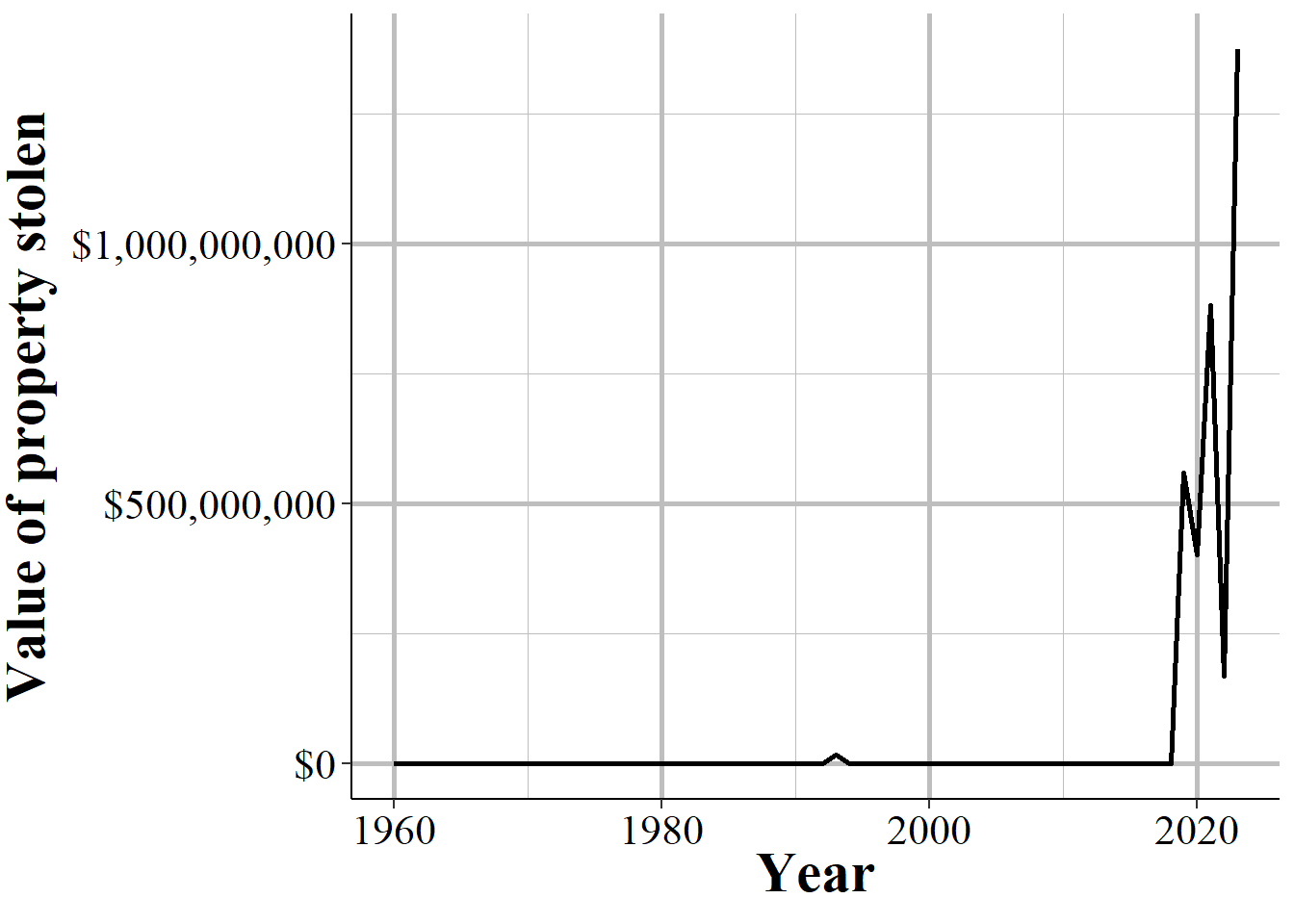
Figure 4.8: The annual value of stolen livestock in New York City, 1960-2023.

It gets harder to determine when a value is a mistake when it is simply a big spike - or drop - in data that otherwise looks correct. Take, for example, the annual value of stolen clothing and fur in Philadelphia from 1960-2019, shown in Figure 4.9. The annual value of these stolen items more than doubled in 1989 compared to the previous year and then declined rapidly in the following year.

Is this real? Is it a data error? It is hard to tell. Here we do not know how many clothing/fur thefts there were, only the value of the total thefts that month (which is aggregated annually here). It continues a multi-year trend of increasing value of thefts but it is larger than previous increases in value. And while the spike is very large in percent terms, it is not so extraordinarily huge that we immediately think it is an error - though some outlier detection methods may think so if it is beyond the expected value for that year.

Philadelphia had several years in this time period where only part of that year’s data was reported. In fact both 1988 and 1989 had fewer than 12 months of data; as did 1974 and 1975. So the year with fewer than 12 months had an atypically high value of clothing and fur stolen. Normally we would expect less data to lead to smaller numbers. But that is not always true. Sometimes less data is a sign that there is something wrong with the data quality altogether and that we need to be cautious of any value in that year. And even though we know that some years are missing months of data just looking at this figure it is not clear which years those are. So while graphing data helps, it is only by looking at the data itself - and yes, this means you will likely need to pull out a programming language like R or python, or at the very least use Excel - and look at each data point before trusting this data.

It is also important to have some understanding of what the data should look like when trying to figure out what data point may be incorrect. In this figure we see a huge spike in 1989. If we know, for example, that a ring of fur thieves were active this year, then that makes it far more likely that the data is real. This may be a rather odd example, but it is helpful to try to understand the context of the data to better understand when the “weird” data is an error and when it is just “weird but right.”

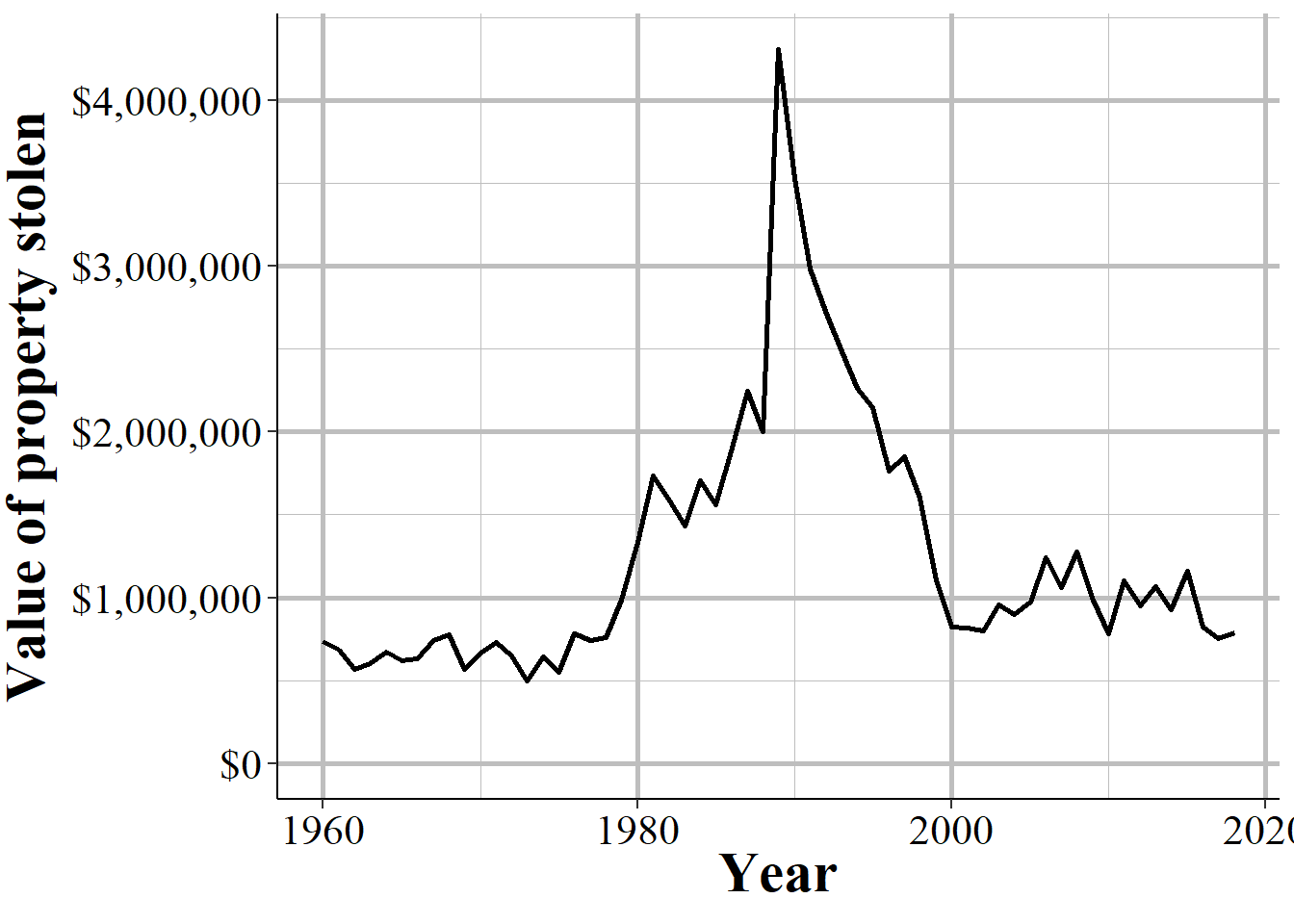
Figure 4.9: The annual value of stolen clothing and fur in Philadelphia, PA, 1960-2019

Finally, some errors are so extreme that it is surprising they were not captured during any of the review points from the police officer entering data in their agency’s computer to the FBI releasing this data to the public. For example, Figure ?? shows Rome, New York, a city of about 32,000 people in central New York State. Here’s what the reported value of bicycles stolen was for Rome in our data.⁴²

2020 had a bit of a spike in their stolen bicycle value, from less than $10,000 is the previous few years to over $5 billion. Yes, that is billion with a “b.” 2021 followed by slightly under $3 billion worth of bicycles stolen. In both years 19 bicycles were reported stolen.

Bicycles were not the only thing stolen in Rome. Consumable goods such as food and toiletries were stolen to the tune of $5 billion in 2020 and $1 billion in 2022, with only $84,278 worth of goods stolen in 2021. To put this into perspective - not that it is needed - the total amount of property stolen by theft the United States during 2019, according to this dataset, was $8 billion. Rome, NY, superseded that by far just through two groups of property stolen in 2020.

Now, obviously this is not real. This is just an error with the police entering in the wrong price. But the issue is that through all the layers of checks that occurred - checks by the local police, by the state UCR system (though some agencies submit directly to the FBI) and the FBI themselves - failed to prevent this incorrect data from being published. This is an obvious, glaring error. If this slipped through the cracks, what less glaring issue did too? So you cannot just trust that this data is right. You need to check and recheck⁴³ everything before using it. This is the right approach for all data, and especially for this data.

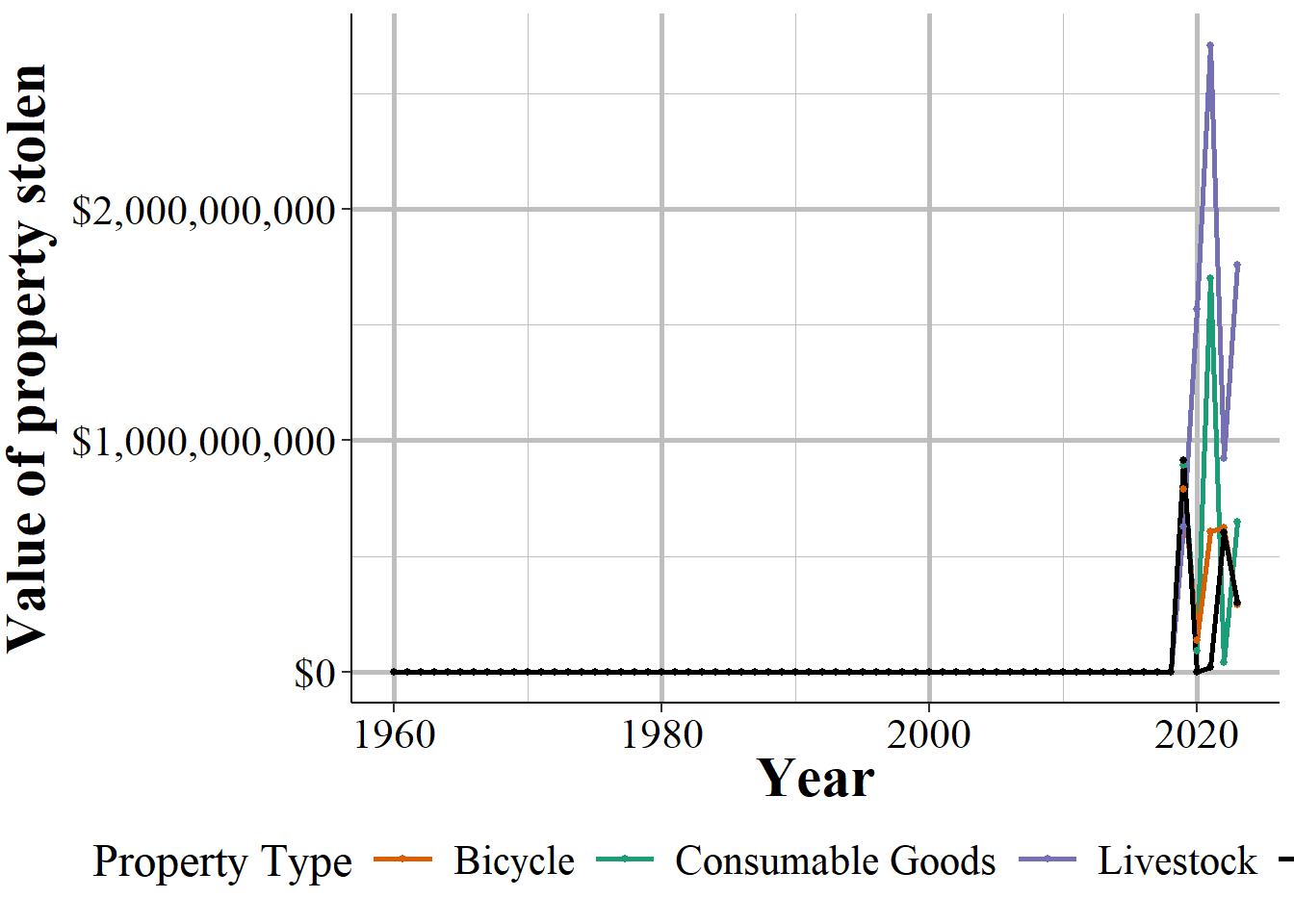
Figure 4.10: The annual value of stolen consumable goods, bicycles, livestock, and thefts from pickpocketing, in Rome, New York, 1960-2023.

The Property Stolen and Recovered dataset offers a useful, though imperfect, view of property crimes and their financial impact. While limitations such as reporting gaps and data inconsistencies exist, careful analysis can still reveal important trends in the types and values of stolen and recovered property. Researchers should approach this data with caution, especially when making year-to-year comparisons or analyzing categories with significant outliers.

---

34. Return A being another name for the Offenses Known and Clearances by Arrest dataset.↩︎

35. Based on the location of the incident - “bank”, “gas station”, etc.↩︎

36. 1974 had11 months, 1975 had 9 months, 1988 had 10 months, and 1989 had 11 months of data.↩︎

37. Having an outlier, as long as it is not just a data entry error, should not necessarily mean you remove it. If we removed rare events after all we would have to drop murders from our data as murders are very uncommon crimes.↩︎

38. Based on June of both years↩︎

39. For more on this process, please see Section 3.4.1↩︎

40. Even if we look at the Offenses Known and Clearances by Arrest data, that only says if there was an arrest or exceptional clearance in the case, not if the property stolen was recovered↩︎

41. Since the minimum value is 0 there is less chance of data errors underestimating the value of an item, though some errors must certainly occur.↩︎

42. For this example we would not worry about years where <12 months of data were reported.↩︎

43. and check again.↩︎