Chapter 2 SRS Overview
One of the first, and most important, questions I think people have about crime is a simple one: is crime going up? Answering it seems simple - you just count up all the crimes that happen in an area and see if that number of bigger than it was in previous times.
However, putting this into practice invites a number of questions, all of which affect how we measure crime. First, we need to define what a crime is. Not philosophically what actions are crimes - or what should be crimes - but literally which of the many thousands of different criminal acts (crimes as defined by state or federal law) should be considered in this measure. Should murder count? Most people would say yes. How about jaywalking or speeding? Many would say probably not. Should marital rape be considered a crime? Now, certainly most people (all, I would hope) would say yes. But in much of the United States it wasn’t a crime until the 1970s (Bennice and Resick 2003; McMahon-Howard, Clay-Warner, and Renzulli 2009).
Next, we have to know what geographic and time unit to measure crimes at since these decisions determine how precise we can measure crime and when it changed. That is, if you are mugged on Jan 1st at exactly 12:15pm right outside your house, how do we record it? Should we be as precise as including the exact time and location (such as your home address)? Out of privacy concerns to the victim, should we only include a larger time unit (such as hour of the day or just the day without any time of day) or a larger geographic unit (such as a Census Tract or the city)?
The final question is that when a crime occurs, how do we know? That is, when we want to count how many crimes occurred do we ask people how often they’ve been victimized, do we ask people how often they commit a crime, do we look at crimes reported to police, crimes charged in a criminal court? Each of these measures will likely give different answers as to how many crimes occurred.
The FBI answered all of these questions in 1929 when they began the Uniform Crime Reporting (UCR) Program Data, or UCR data for short. Crime consists of eight crime categories - murder, rape, robbery, aggravated assault, burglary, motor vehicle theft, theft, and simple assault - that are reported to the police and is collected each month from each agency in the country. So essentially we know how many of a small number of crime categories happen each month in each city (though some cities have multiple police agencies so even this is more complicated than it seems). These decisions, born primarily out of the resource limitations of 1929 (i.e. no computers), have had a major impact on criminology research. The first seven crime categories - known as “Index Crimes” or “Part 1 crimes” (or “Part I” sometimes) - are the ones used to measure crime in many criminology papers, even when the researchers have access to data that covers a broader selection of crimes than these.6 These are also the crimes that the news uses each year to report on how crime in the United States compares to the previous year. The crime data actually also includes the final crime, simple assault, though it is not included as an index crime and is, therefore, generally ignored by researchers - a relatively large flaw in most studies that we’ll discuss in more detail in Section 2.1.3.
2.1 Crimes included in the UCR data sets
UCR data covers only a subset - and for the crime data, a very small subset - of all crimes that can occur. It also only includes crimes reported to the police. So there are two levels of abstraction from a crime occurring to it being included in the data: a crime must occur that is one of the crimes included in one of the UCR data sets (we detail all of these crimes below) and the victim must report the incident to the police. While the crimes included are only a small selection of crimes - which were originally chosen since at the time the UCR was designed these were considered important offenses and among the best reported - this is an important first step to understanding the data.
UCR data should be understood as a loose collection of data that seeks to understand crimes and arrests in the United States. There are seven data sets in the UCR collection that each cover a different topic or a subset of a previously covered topic: crimes, arrests, property crimes specifically, homicides specifically, police officers killed or assaulted, arson specifically, and hate crimes.7 In this section we’ll go over the crimes included in the two main UCR data sets: Offenses Known and Clearances by Arrest and (which I like to call the “crime” data set) and the Arrests by Age, Sex, and Race (the “arrests” data set). These are the most commonly used UCR data sets and the stolen property and homicide data sets are simply more detailed subsets of these data sets. The hate crime data set can cover a broader selection of offenses than in the crimes or arrests data, so we’ll discuss those in the hate crimes chapter.
2.1.1 Crimes in the Offenses Known and Clearances by Arrest data set
As mentioned above - and as most criminology papers will tell you - the crimes included in the UCR’s Offenses Known and Clearances by Arrest data are the seven index crimes (eight when including arson, though arson is only reported in its own data set so is usually excluded) - homicide, rape, robbery, aggravated assault, burglary, theft, and motor vehicle theft - as well as simple assault. This is true but incomplete. The data also includes subcategories for all crimes other than simple assault and theft - though theft has its own UCR data set which goes into detail about the thefts. Both robbery and aggravated assault, for example, have subcategories showing which weapon the offender used (if any) during the crime. This allows for a more detailed understanding of the crime than looking only at the broad category. I’m not sure why most research includes only the broader categories and doesn’t tend to look at subcategories, but that seems to be the case in most studies that I have read. Some police agencies only report the broader categories and don’t report subcategories, but most report subcategories so this is an under-exploited source of data.
- Homicide
- Murder and non-negligent manslaughter
- Manslaughter by negligence
- Rape
- Completed rape
- Attempted rape
- Robbery
- With a firearm
- With a knife of cutting instrument
- With a dangerous weapon not otherwise specified
- Unarmed - using hands, fists, feet, etc.
- Aggravated Assault (assault with a weapon or with the intent to cause serious bodily injury)
- With a firearm
- With a knife of cutting instrument
- With a dangerous weapon not otherwise specified
- Unarmed - using hands, fists, feet, etc.
- Burglary
- With forcible entry
- Without forcible entry
- Attempted burglary with forcible entry
- Theft (other than of a motor vehicle)
- Motor vehicle theft
- Theft of a car
- Theft of a truck or bus
- Theft of an other type of vehicle
- Simple Assault
2.1.2 Crimes in the Arrests by Age, Sex, and Race data set
The crimes included in the Arrests by Age, Sex, and Race - the “arrest” data tells you how many people were arrested for a particular crime category - are different than those in the crime data. The arrest data covers a wider variety of crimes, including drug and alcohol crimes, gambling, and fraud. However, it is also less detailed than the crime data set when it comes to violent crime. While it covers the same broad categories of violent crimes as the crimes data - murder, rape, robbery, aggravated assault, and simple assault - it doesn’t include the more detailed breakdown that is available in the crime data. For example, in the crime data robbery is included as well as the subcategories of robbery with a gun, robbery with a knife, robbery with another dangerous weapon, and robbery without a weapon. In comparison, the arrest data only includes robbery without any subcategories.
- Homicide
- Murder and non-negligent manslaughter
- Manslaughter by negligence
- Rape
- Robbery
- Aggravated assault
- Burglary
- Theft (other than of a motor vehicle)
- Motor vehicle theft
- Simple assault
- Arson
- Forgery and counterfeiting
- Fraud
- Embezzlement
- Stolen property - buying, receiving, and possessing
- Vandalism
- Weapons offenses - carrying, possessing, etc.
- Prostitution and commercialized vice
- Sex offenses - other than rape or prostitution
- Drug abuse violations - total
- Drug sale or manufacturing
- Opium and cocaine, and their derivatives (including morphine and heroin)
- Marijuana
- Synthetic narcotics
- Other dangerous non-narcotic drugs
- Drug possession
- Opium and cocaine, and their derivatives (including morphine and heroin)
- Marijuana
- Synthetic narcotics
- Other dangerous non-narcotic drugs
- Gambling - total
- Bookmaking - horse and sports
- Number and lottery
- All other gambling
- Offenses against family and children - nonviolent acts against family members. Includes neglect or abuse, nonpayment of child support or alimony.
- Driving under the influence (DUI)
- Liquor law violations - Includes illegal production, possession (e.g. underage) or sale of alcohol, open container, or public use laws. Does not include DUIs and drunkenness.
- Drunkenness - i.e. public intoxication
- Disorderly conduct
- Vagrancy - includes begging, loitering (for adults only), homelessness, and being a “suspicious person.”
- All other offenses (other than traffic) - a catch-all category for any arrest that is not otherwise specified in this list. Does not include traffic offenses. Very wide variety of crimes are included - use caution when using!
- Suspicion - “Arrested for no specific offense and released without formal charges being placed.”
- Curfew and loitering law violations - for minors only.
- Runaways - for minors only.
2.1.3 What is an index (or part 1) crime?
One of the first (and seemingly only) thing that people tend to learn about UCR crime data is that it covers something called an “index crime.”8 Index crimes, sometimes written as Part 1 or Part I crimes, are the seven crimes originally chosen by the FBI to be included in their measure of crimes as these offenses were both considered serious and generally well-reported so would be a useful measure of crime. Index crimes are often broken down into property index crimes - burglary, theft, and motor vehicle theft (and arson now, though that’s often not included and is reported less often by agencies) - and violent index crimes (murder, rape, robbery, and aggravated assault). The “index” is simply that all of the crimes are summed up into a total count of crimes (violent, property, or total) for that police agency.
The biggest problem with index crimes is that it is simply the sum of 8 (or 7 since arson data usually isn’t included) crimes. Index crimes have a huge range in their seriousness - it includes, for example, both murder and theft - so summing up the crimes gives each crime equal weight. This is clearly wrong as 100 murders is more serious than 100 thefts. This is especially a problem as less serious crimes (theft mostly) are far more common than more serious crimes. In 2017, for example, there were 1.25 million violent index crimes in the United States. That same year had 5.5 million thefts. So using index crimes as your measure of crimes fails to account for the seriousness of crimes. Looking at total index crimes is, in effect, mostly just looking at theft. Looking at violent index crimes alone mostly measures aggravated assault. This is especially a problem because it hides trends in violent crimes. As an example, San Francisco, shown in Figure 2.1, has had a huge increase - about 50% - in index crimes in the last several years. When looking closer, that increase is driven almost entirely by the near doubling of theft since 2011. During the same years, index violent crimes have stayed fairly steady. So the city isn’t getting more dangerous - at least not in terms of violent index crimes increasing - but it appears like it is due to just looking at total index crimes.
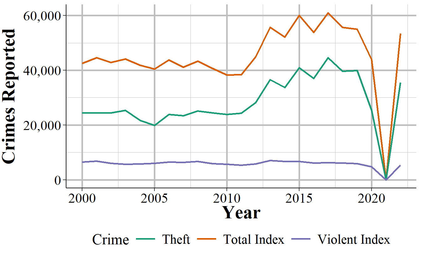
Figure 2.1: Thefts and total index crimes in San Francisco, 2000-2022.
Many researchers divide index crimes into violent and nonviolent categories, which helps but even this isn’t entirely sufficient. Take Chicago as an example. It is a city infamous for its large number of murders. But as a fraction of index crimes, Chicago has a rounding error worth of murders. Their 653 murders in 2017 is only 0.5% of total index crimes. For violent index crimes, murder made up 2.2% of crimes that year. As seen in Figure 2.2, in no year where data is available did murders account for more than 3.5% of violent index crimes; and, while murders are increasing as a percent of violent index crimes they still account for no more than 2.5% in most recent years. What this means is that changes in murder are very difficult to detect. If Chicago had no murders this year, but a less serious crime (such as theft) increased slightly, we couldn’t tell from looking at the number of index crimes, even from violent index crimes. As discussed in the below section, using this sample of crimes as the primary measure of crimes - and particularly of violent crimes - is also misleading as it excludes important - and highly common relative to index crimes - offenses, such as simple assault.
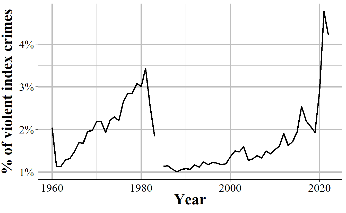
Figure 2.2: Murders in Chicago as a percent of violent index crimes, 1960-2022.
2.1.3.1 What is a violent crime?
An important consideration in using this data is defining what a “violent crime” is. One definition, and the one that I think makes the most sense, is that a violent crime is one that uses force or the threat of force. For example, if I punch you in the face, that is a violent crime. If I stab you, that is a violent crime. While clearly different in terms of severity, both incidents used force so I believe would be classified as a violent crime. The FBI, and most researchers, reporters, and advocates would disagree. Organizations ranging from the FBI itself to Pew Research Center and advocacy groups like the Vera Institute of Justice and the ACLU all define the first example as a non-violent crime and the second as a violent crime. They do this for three main reasons.
The first reason is that simple assault is not an index crime, so they don’t include it when measuring violent crime. It is almost a tautology in criminology that you use index crimes as the measure of crime since that’s just what people do. As far as I’m aware, this is really the main reason why researchers justify using index crimes: because people in the past used it so that’s just what is done now.9 This strikes me as a particularly awful way of doing anything, more so since simple assault data has been available almost as long as index crime data.10
The second reason - and one that I think makes sense for reporters and advocates who are less familiar with the data, but should be unacceptable to researchers - is that people don’t know that simple assault is included, or at least don’t have easy access to it. Neither the FBI’s annual report page not their official crime data tool website include simple assault since they only include index crimes. For people who rely only on these sources - and given that using the data itself requires at least some programming skills, I think this accounts for most users and certainly nearly all non-researchers - it is not possible to access simple assault crime data (arrest data does include simple assault on these sites) from these official sources.
The final reason is that it benefits some people’s goals to classify violent crime as only including index crimes. This is because simple assault is extremely common compared to violent index crimes - in many cities simple assault is more common than all violent index crimes put together - so excluding simple assault makes it seem like fewer arrests are violent than they are when including simple assault. For example, a number of articles have noted that marijuana arrests are more common than violent crime arrests (Ingraham 2016; Kertscher 2019; Devito 2020; Earlenbaugh 2020; Edwards et al. 2020) or that violent crime arrests are only 5% of all arrests (Neusteter and O’Toole 2019; Speri 2019).11 While true when considering only violent index crimes, including simple assault as a violent crime makes these statements false. Some organizations call the violent index crimes “serious violent crimes” which is an improvement but even this is a misnomer since simple assault can lead to more serious harm than aggravated assault. An assault becomes aggravated if using a weapon or there is the potential for serious harm, even if no harm actually occurs.12
As an example of this last point, Figure 2.3 shows the number of violent index crimes and simple assaults each year from 1960 to 2018 in Houston, Texas (simple assault is not reported in UCR until 1964, which is why 1960-1963 show zero simple assaults). In every year where simple assault is reported, there are more simple assaults than aggravated assaults. Beginning in the late 1980s, there are also more simple assaults than total violent index crimes. Excluding simple assault from being a violent crime greatly underestimates violence in the country.
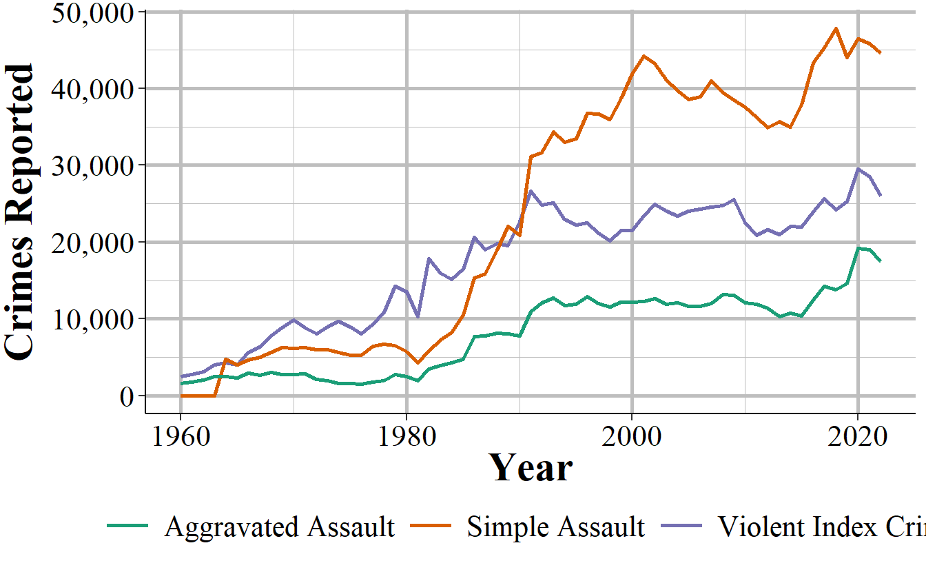
Figure 2.3: Reported crimes in Houston, Texas, from 1960 to 2018. Violent index crimes are aggravated assault, rape, robbery, and murder.
2.2 Issues common across UCR data sets
In this section we’ll discuss issues common to most or all of the UCR data sets. For some of these, we’ll come back to the issues in more detail in the chapter for the data sets most affected by the problem.
2.2.1 Negative numbers
One of the most common questions people have about this data is why there are negative numbers, and if they are a mistake. Negative numbers are not a mistake. The UCR data is monthly so police agencies report the number of monthly crimes that are known to them - either reported to them or discovered by the police. In some cases the police will determine that a crime reported to them didn’t actually occur - which they called an “unfounded crime.” An example that the FBI gives for this is a person reports their wallet stolen (a theft) and then later finds it, so a crime was initially reported but no crime actually occurred.
How this works when the police input the data is that an unfounded crime is reported both as an unfounded crime and as a negative actual crime - the negative is used to zero out the erroneous report of the actual crime. So the report would look like 1 actual theft (the crime being reported), -1 theft (the crime being discovered as not have happened), and 1 unfounded theft. If both incidents occurred in the same month then this would simply be a single unfounded theft occurring, with no actual theft - literally a value of 1 + -1 = 0 thefts.
Negative values occur when the unfounding happens in a later month than the crime report. In the theft case, let’s say the theft occurred in January and the discovery of the wallet happens in August. Assuming no other crimes occurred, January would have 1 theft, and August would have -1 thefts and 1 unfounded theft. There is no way of determining in which month (or even which year) an unfounded crime was initially reported in. When averaging over the long term, there shouldn’t be any negative numbers as the actual and unfounded reports will cancel themselves out. However, when looking at monthly crimes - particularly for rare crimes - you’ll still see negative numbers for this reason. Since crimes can be unfounded for reports in previous years, you can actually see entire year’s crime counts be negative, though this is much rarer than monthly values.13
2.2.2 Agency population value
Each of the UCR data sets include a population variable that has the estimated population under the jurisdiction of that agency.14 This variable is often used to create crime rates that control for population. In cases where jurisdiction overlaps, such as when a city has university police agencies or county sheriffs in counties where the cities in that county have their own police, UCR data assigns the population covered to the most local agency and zero population to the overlapping agency. So an agency’s population is the number of people in that jurisdiction that isn’t already covered by a different agency.
For example, the city of Los Angeles in California has nearly four million residents according to the US Census. There are multiple police agencies in the city, including the Los Angeles Police Department, the Los Angeles County Sheriff’s Office, the California Highway Patrol that operates in the area, airport and port police, and university police departments. If each agency reported the number of people in their jurisdiction - which all overlap with each other - we would end up with a population far higher than LA’s four million people. To prevent double-counting population when agency’s jurisdictions overlap, the non-primary agency will report a population of 0, even though they still report crime data like normal. As an example, in 2018 the police department for California State University - Los Angeles reported 92 thefts and a population of 0. Those 92 thefts are not counted in the Los Angeles Police Department data, even though the department counts the population. To get complete crime counts in Los Angeles, you’d need to add up all police agencies within in the city; since the population value is 0 for non-LAPD agencies, both the population and the crime sum will be correct.
The UCR uses this method even when only parts of a jurisdiction overlaps. Los Angeles County Sheriff has a population of about one million people, far less than the actual county population (the number of residents, according to the Census) of about 10 million people. This is because the other nine million people are accounted for by other agencies, mainly the local police agencies in the cities that make up Los Angeles County.
The population value is the population who reside in that jurisdiction and does not count people who are in the area but don’t live there, such as tourists or people who commute there for work. This means that using the population value to determine a rate can be misleading as some places have much higher numbers of non-residents in the area (e.g. Las Vegas, Washington D.C.) than others.
2.2.3 Reporting is voluntary … so some agencies don’t (or report partially)
When an agency reports their data to the FBI, they do so voluntarily - there is no national requirement to report.15 This means that there is inconsistency in which agencies report, how many months of the year they report for, and which variables they include in their data submissions.
In general, more agencies report their data every year and once an agency begins reporting data they tend to keep reporting. The UCR data sets are a collection of separate, though related, data sets and an agency can report to as many of these data sets as they want - an agency that reports to one data set does not mean that they report to other data sets. Figure 2.4 shows the number of agencies that submitted at least one month of data to the Offenses Known and Clearances by Arrest data in the given year. For the first decade of available data under 8,000 agencies reported data and this grew to over 13,500 by the late 1970s before plateauing for about a decade. The number of agencies that reported their data actually declined in the 1990s, driven primarily by many Florida agencies temporarily dropping out, before growing steadily to nearly 17,000 agencies in 2010; from here it kept increasing but slower than before.
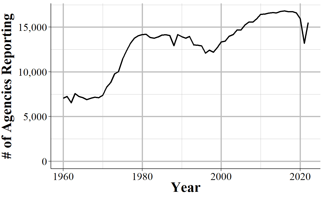
Figure 2.4: The annual number of agencies reporting to the Offenses Known and Clearances by Arrest data set. Reporting is based on the agency reporting at least one month of data in that year.
There are approximately 18,000 police agencies in the United States so recent data has reports from nearly all agencies, while older data has far fewer agencies reporting. When trying to estimate to larger geographies, such as state or national-level, later years will be more accurate as you’re missing less data. For earlier data, however, you’re dealing with a smaller share of agencies meaning that you have a large amount of missing data and a less representative sample.
Figure 2.5 repeats the above figure but now including only agencies with 100,000 people or more in their jurisdiction. While these agencies have a far more linear trend than all agencies, the basic lesson is the same: recent data has most agencies reporting; old data excludes many agencies.
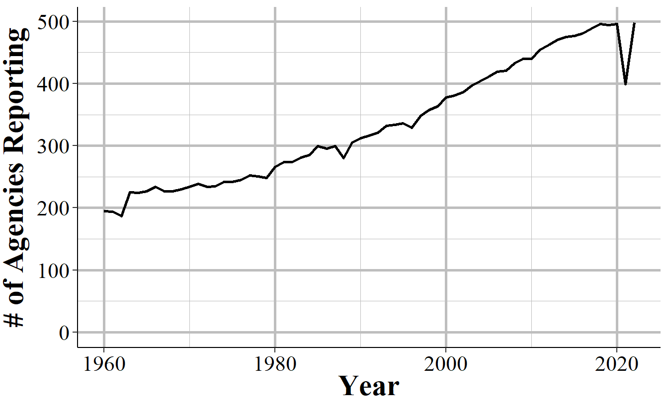
Figure 2.5: The annual number of agencies with a population of 100,000 or higher reporting to the Offenses Known and Clearances by Arrest data set. Reporting is based on the agency reporting at least one month of data in that year.
This voluntariness extends beyond whether they report or not, but into which variables they report. While in practice most agencies report every crime when they report any, they do have the choice to report only a subset of offenses. This is especially true for subsets of larger categories - such as gun assaults, a subset of aggravated assaults, or marijuana possession arrests which is a subset of drug possession arrests. As an example, Figure 2.6 shows the annual number of aggravated assaults with a gun in New York City. In 2003 the New York Police Department stopped reporting this category of offense, resuming only in 2013. They continued to report the broader aggravated assault category, but not any of the subsections of aggravated assaults which say which weapon was used during the assault.
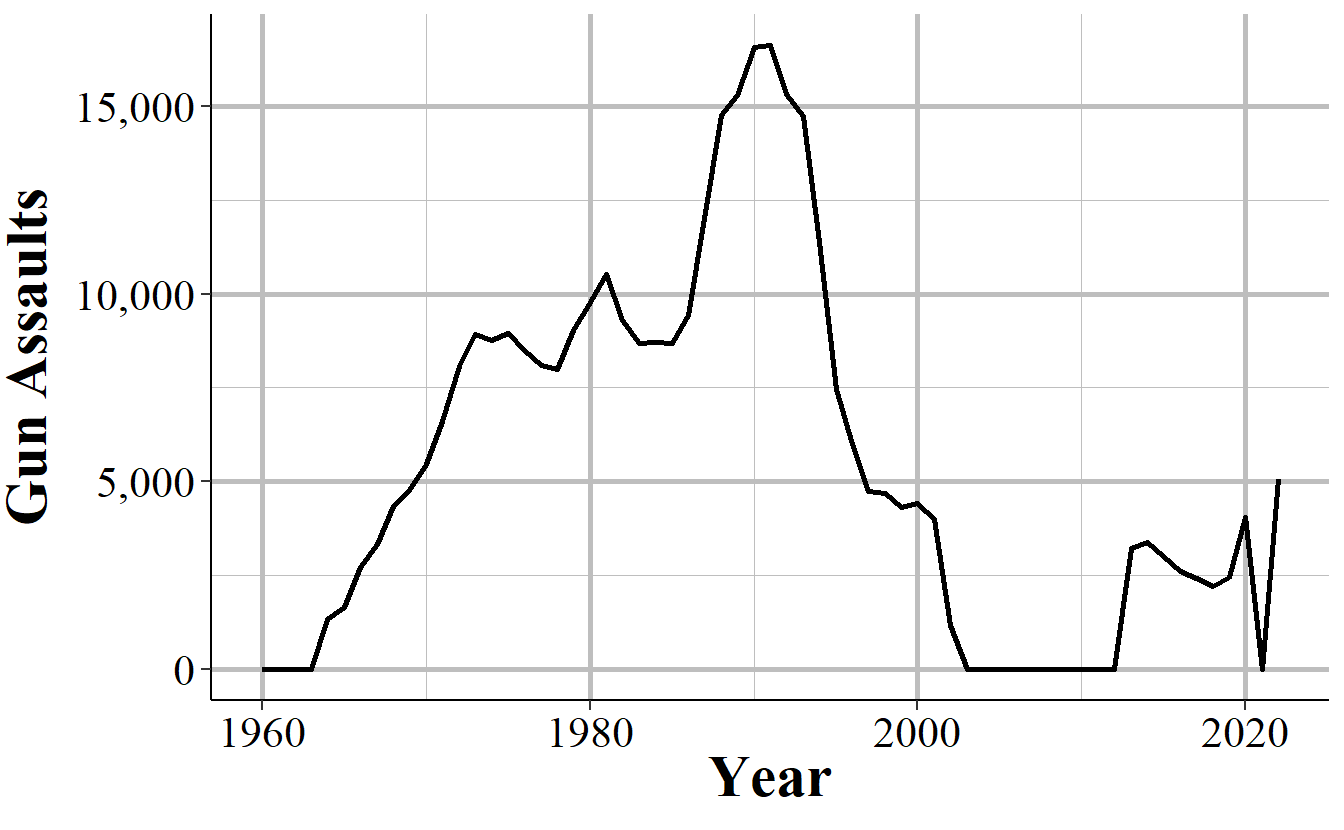
Figure 2.6: Monthly reports of gun assaults in New York City, 1960-2022.
Given that agencies can join or drop out of the UCR program at will, and report only partial data, it is highly important to carefully examine your data to make sure that there are no issues caused by this.
Even when an agency reports UCR data, and even when they report every crime category, they can report fewer than 12 months of data. In some cases they simply report all of their data in December, or report quarterly or semi-annually so some months have zero crimes reported while others count multiple months in that month’s data. One example of this is New York City, shown in Figure 2.7, in the early-2000s to the mid-2010s where they began reporting data quarterly instead of monthly.
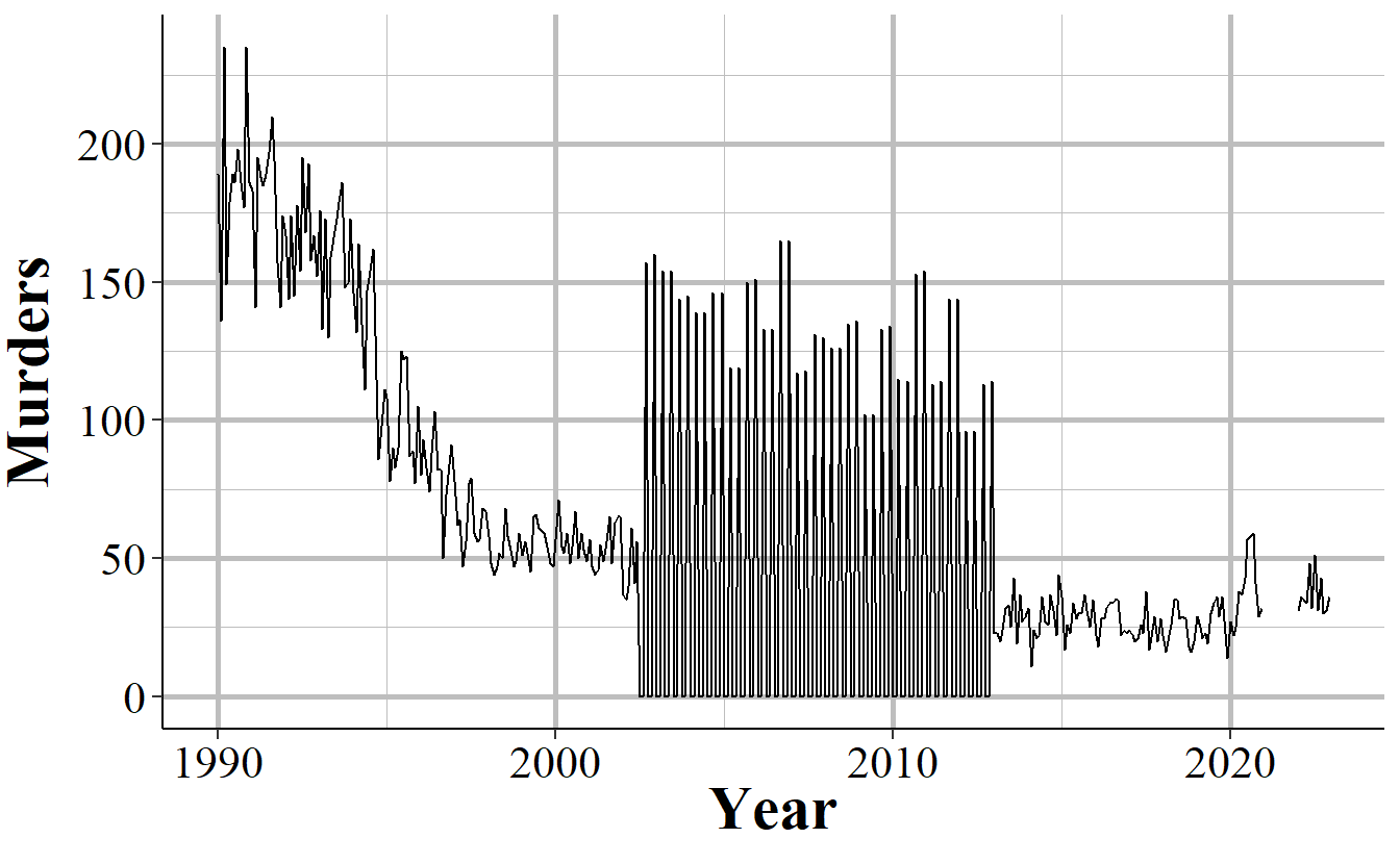
Figure 2.7: Monthly murders in New York City, 1990-2022. During the 2000s, the police department began reporting quarterly instead of monthly and then resumed monthly reporting.
When you sum up each month into an annual count, as shown in Figure 2.8, the problem disappears since the zero months are accounted for in the months that have the quarterly data. If you’re using monthly data and only examine the data at the annual level, you’ll fall into the trap of having incorrect data that is hidden due to the level of aggregation examined. While cases like NYC are obvious when viewed monthly, for people that are including thousands of agencies in their data, it is unfeasible to look at each agency for each crime included. This can introduce errors as the best way to examine the data is manually viewing graphs and the automated method, looking for outliers through some kind of comparison to expected values, can be incorrect.
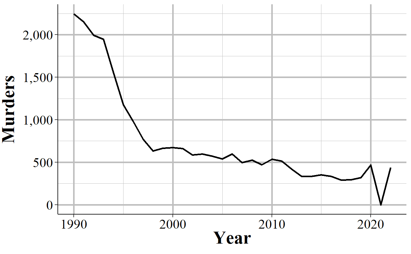
Figure 2.8: Annual murders in New York City, 1990-2022.
In other cases when agencies report fewer than 12 months of the year, they simply report partial data and as a result undercount crimes. Figure 2.9 shows annual murders in Miami-Dade, Florida and has three years of this issue occurring. The first two years with this issue are the two where zero murders are reported - this is because the agency didn’t report any months of data. The final year is in 2018, the last year of data in this graph, where it looks like murder suddenly dropped significantly. That’s just because Miami-Dade only reported through June, so they’re missing half of 2018.
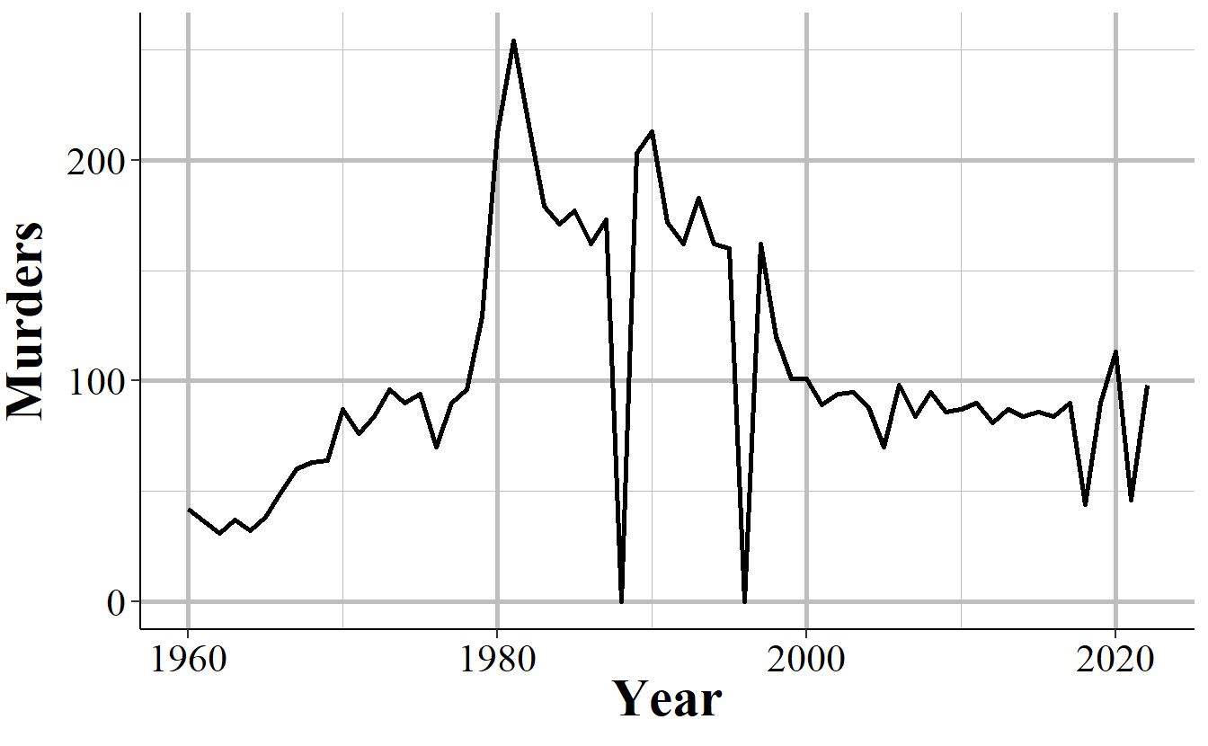
Figure 2.9: Annual murders in Miami-Dade, Florida, 1960-2022.
2.2.4 Zero crimes vs no reports
When an agency does not report, we see it in the data as reporting zero crimes, not reporting NA or any indicator that they did not report. In cases where the agency says they didn’t report that month we can be fairly sure (not entirely since that variable isn’t always accurate) that the zero crimes reported are simply that the agency didn’t report. In cases where the agency says they report that month but report zero crimes, we can’t be sure if that’s a true no crimes reported to the agency or the agency not reporting to the UCR. As agencies can report some crimes but not others in a given month and still be considered reporting that month, just saying they reported doesn’t mean that the zero is a true zero.
In some cases it is easy to see when a zero crimes reported is actually the agency not reporting. As Figure 2.6 shows with New York City gun assaults, there is a massive and sustained dropoff to zero crimes and then a sudden return years later. Obviously, going from hundreds of crimes to zero crimes is not a matter of crimes not occurring anymore, it is a matter of the agency not reporting - and New York City did report other crimes these years so in the data it says that they reported every month. So in agencies which tend to report many crimes - and many here can be a few as 10 a year since going from 10 to 0 is a big drop - a sudden report of zero crimes is probably just non-reporting.
Differentiating zero crimes and no reports becomes tricky in agencies that tend to report few crimes, which most small towns do. As an example, Figure 2.10 shows the annual reports of rape in Danville, California, a city of approximately 45,000 people. The city reports on average 2.8 rapes per year and in five years reported zero rapes. In cases like this it’s not clear whether we should consider those zero years as true zeros (that no one was raped or reported their rape to the police) or whether the agency simply didn’t report rape data that year.
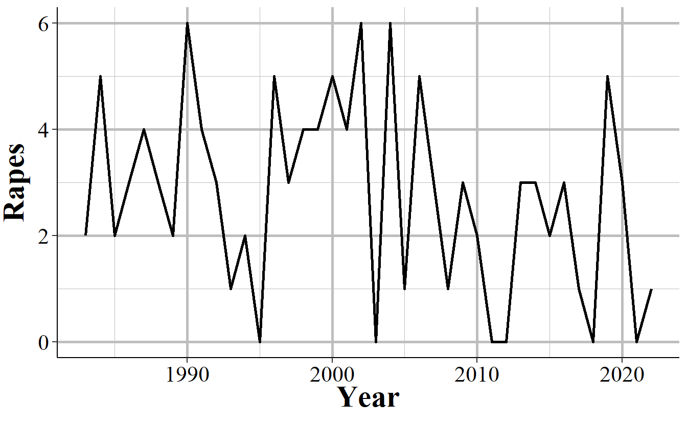
Figure 2.10: Annual rapes reported in Danville, CA, 1960-2022.
2.3 A summary of each UCR data set
The UCR collection of data can be roughly summarized into two groups: crime data and arrest data. While there are several data sets included in the UCR data collection, they are all extensions of one of the above groups. For arrest data, you have information about who (by race and by age-gender, but not by race-gender or race-age other than within race you know if the arrestee is an adult or a juvenile) was arrested for each crime. For crime data, you have monthly counts of a small number of crimes (many fewer than crimes covered in the arrest data) and then more specialized data on a subset of these crimes - information on homicides, hate crimes, assaults or killings of police officers, and stolen property.
Each of these data sets will have its own chapter in this book where we discuss the data thoroughly. Here is a very brief summary of each data set which will help you know which one to use for your research. I still recommend reading that data’s chapter since it covers important caveats and uses (or misuses) of the data that won’t be covered below.
2.3.1 Offenses Known and Clearances by Arrest
The Offenses Known and Clearances by Arrest data set - often called Return A, “Offenses Known” or, less commonly, OKCA - is the oldest and most commonly used data set and measures crimes reported to the police. For this reason it is used as the main measure of crime in the United States, and I tend to call it the “crimes data set.” This data includes the monthly number of crimes reported to the police or otherwise known to the police (e.g. discovered while on patrol) for a small selection of crimes, as well as the number of crimes cleared by arrest or by “exceptional means” (a relatively flawed and manipulable measure of whether the case is “solved”). It also covers the number reported but found by police to have not occurred. Since this data has monthly agency-level crime information it is often used to measure crime trends between police agencies and over time. The data uses something called a Hierarchy Rule which means that in incidents with multiple crimes, only the most serious is recorded - though in practice this affects only a small percent of cases, and primarily affects property crimes.
2.3.2 Arrests by Age, Sex, and Race
The Arrests by Age, Sex, and Race data set - often called ASR or the “arrests data” - includes the monthly number of arrests for a variety of crimes and, unlike the crime data, breaks down this data by age and gender. This data includes a broader number of crime categories than the crime data set (the Offenses Known and Clearances by Arrest data) though is less detailed on violent crimes since it does not breakdown aggravated assault or robberies by weapon type as the Offenses Known data does. For each crime it says the number of arrests for each gender-age group with younger ages (15-24) showing the arrestee’s age to the year (e.g. age 16) and other ages grouping years together (e.g. age 25-29, 30-34, “under 10”). It also breaks down arrests by race-age by including the number of arrestees of each race (American Indian, Asian, Black, and White are the only included races) and if the arrestee is a juvenile (<18 years old) or an adult. The data does technically include a breakdown by ethnicity-age (e.g. juvenile-Hispanic, juvenile-non-Hispanic) but almost no agencies report this data (for many years zero agencies report ethnicity) so in practice the data does not include ethnicity. As the data includes counts of arrestees, people who are arrested multiple times are included in the data multiple times - it is not a measure of unique arrestees.
2.3.3 Law Enforcement Officers Killed and Assaulted (LEOKA)
The Law Enforcement Officers Killed and Assaulted data, often called just by its acronym LEOKA, has two main purposes.16 First, it provides counts of employees employed by each agency - broken down by if they are civilian employees or sworn officers, and also broken down by gender. And second, it measures how many officers were assaulted or killed (including officers who die accidentally such as in a car crash) in a given month. The assault data is also broken down into shift type (e.g. alone, with a partner, on foot, in a car, etc.), the offender’s weapon, and type of call they are responding to (e.g. robbery, disturbance, traffic stop). The killed data simply says how many officers are killed feloniously (i.e. murdered) or died accidentally (e.g. car crash) in a given month. The employee information is at the year-level so you know, for example, how many male police officers were employed in a given year at an agency, but don’t know any more than that such as if the number employed changed over the year. This data set is commonly used as a measure of police employees and is a generally reliable measure of how many police are employed by a police agency. The second part of this data, measuring assaults and deaths, is more flawed with missing data issues and data error issues (e.g. more officers killed than employed in an agency).
2.3.4 Supplementary Homicide Reports (SHR)
The Supplementary Homicide Reports data set - often abbreviated to SHR - is the most detailed of the UCR data sets and provides information about the circumstances and participants (victim and offender demographics and relationship status) for homicides.17 For each homicide incident it tells you the age, gender, race, and ethnicity of each victim and offender as well as the relationship between the first victim and each of the offenders (but not the other victims in cases where there are multiple victims). It also tells you the weapon used by each offender and the circumstance of the killing, such as a “lovers triangle” or a gang-related murder. As with other UCR data, it also tells you the agency it occurred in and the month and year when the crime happened.
2.3.5 Hate Crime Data
This data set covers crimes that are reported to the police and judged by the police `to be motivated by hate. More specifically, they are, first, crimes which were, second, motivated - at least in part - by bias towards a certain person or group of people because of characteristics about them such as race, sexual orientation, or religion. The first part is key, they must be crimes - and really must be the selection of crimes that the FBI collects for this data set. Biased actions that don’t meet the standard of a crime, or are of a crime not included in this data, are not considered hate crimes. For example, if someone yells at a Black person and uses racial slurs against them, it is clearly a racist action. For it to be included in this data, however, it would have to extend to a threat since “intimidation” is a crime included in this data but lesser actions such as simply insulting someone is not included. For the second part, the bias motivation, it must be against a group that the FBI includes in this data. For example, when this data collection began crimes against transgender people were not counted so if a transgender person was assaulted or killed because they were transgender, this is not a hate crime recorded in the data (though it would have counted in the “Anti-Lesbian, Gay, Bisexual, Or Transgender, Mixed Group (LGBT)” bias motivation which was always reported).18
So this data is really a narrower measure of hate crimes than it might seem. In practice it is (some) crimes motivated by (some) kinds of hate that are reported to the police. It is also the most under-reported UCR data set with most agencies not reporting any hate crimes to the FBI. This leads to huge gaps in the data with some states having extremely few agencies reporting crime - see, for example Figure 2.11 for state-level hate crimes in 2018 - agencies reporting some bias motivations but not others, agencies reporting some years but not others. While these problems exist for all of the UCR data sets, it is most severe in this data. This problem is exacerbated by hate crimes being rare even in agencies that report them - with such rare events, even minor changes in which agencies report or which types of offenses they include can have large effects.
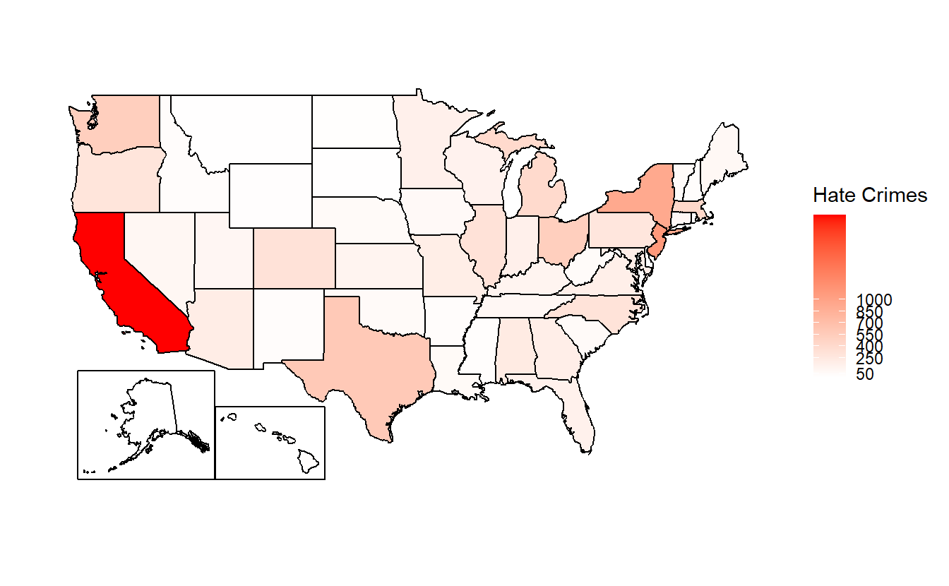
Figure 2.11: Total reported hate crimes by state, 2022.
2.3.6 Property Stolen and Recovered (Supplement to Return A)
The Property Stolen and Recovered data - sometimes called the Supplement to Return A (Return A being another name for the Offenses Known and Clearances by Arrest data set, the “crime” data set) - provides monthly information about property-related offenses (theft, motor vehicle theft, robbery, and burglary), including the location of the offense (in broad categories like “gas station” or “residence”), what was stolen (e.g. clothing, livestock, firearms), and how much the stolen items were worth.19 The “recovered” part of this data set covers the type and value of property recovered so you can use this, along with the type and value of property stolen, to determine what percent and type of items the police managed to recover. Like other UCR data sets this is at the agency-month level so you can, for example, learn how often burglaries occur at the victim’s home during the day, and if that rate changes over the year or differs across agencies. The data, however, provides no information about the offender or the victim (other than if the victim was an individual or a commercial business [based on the location of the incident - “bank”, “gas station”, etc.]). The value of the property stolen is primarily based on the victim’s estimate of how much the item is worth (items that are decreased in value once used - such as cars - are supposed to be valued at the current market rate, but the data provides no indication of when it uses the current market rate or the victim’s estimate) so it should be used as a very rough estimate of value.
2.3.7 Arson
The arson data set provides monthly counts at the police agency-level for arsons that occur, and includes a breakdown of arsons by the type of arson (e.g. arson of a person’s home, arson of a vehicle, arson of a community/public building) and the estimated value of the damage caused by the arson. This data includes all arsons reported to the police or otherwise known to the police (e.g. discovered while on patrol) and also has a count of arsons that lead to an arrest (of at least one person who committed the arson) and reports that turned out to not be arsons (such as if an investigation found that the fire was started accidentally).
For each type of arson it includes the number of arsons where the structure was uninhabited or otherwise not in use, so you can estimate the percent of arsons of buildings which had the potential to harm people. This measure is for structures where people normally did not inhabit the structure - such as a vacant building where no one lives. A home where no one is home at the time of the arson does not count as an uninhabited building.
In cases where the arson led to a death, that death would be recorded as a murder on the Offenses Known and Clearances by Arrest data set - but not indicated anywhere on this data set. If an individual who responds to the arson dies because of it, such as a police officer or a firefighter, this is not considered a homicide (though the officer death is still included in the Law Enforcement Officers Killed and Assaulted data) unless the arsonist intended to cause their deaths. Even though the UCR uses the Hierarchy Rule, where only the most serious offense that occurs is recorded, all arsons are reported - arson is exempt from the Hierarchy Rule.
2.4 How to identify a particular agency (ORI codes)
In the UCR and other FBI data sets, agencies are identified using ORiginating Agency Identifiers or an ORI. An ORI is a unique ID code used to identify an agency.20 If we used the agency’s name we’d end up with some duplicates since there can be multiple agencies in the country (and in a state, those this is very rare) with the same name. For example, if you looked for the Philadelphia Police Department using the agency name, you’d find both the “Philadelphia Police Department” in Pennsylvania and the one in Mississippi. Each ORI is a 7-digit value starting with the state abbreviation (for some reason the FBI incorrectly puts the abbreviation for Nebraska as NB instead of NE) followed by 5 numbers.21 When dealing with specific agencies, make sure to use the ORI rather than the agency name to avoid any mistakes.
For an easy way to find the ORI number of an agency, use this page on my site. Type an agency name or an ORI code into the search section and it will return everything that is a match.
2.5 The data as you get it from the FBI
We’ll finish this overview of the UCR data by briefly talking about format of the data that is released by the FBI, before the processing done by myself or NACJD that converts the data to a type that software like R or Stata or Excel can understand. The FBI releases their data as fixed-width ASCII files which are basically just an Excel file but with all of the columns squished together. As an example, Figure 11.5 shows what the data looks like as you receive it from the FBI for the Offenses Known and Clearances by Arrest data set for 1960, the first year with data available. In the figure, it seems like there are multiple rows but that’s just because the software that I opened the file in isn’t wide enough - in reality what is shown is a single row that is extremely wide because there are over 1,500 columns in this data. If you scroll down enough you’ll see the next row, but that isn’t shown in the current image. What is shown is a single row with a ton of columns all pushed up next to each other. Since all of the columns are squished together (the gaps are just blank spaces because the value there is a space, but that doesn’t mean there is a in the data. Spaces are possible values in the data and are meaningful), you need some way to figure out which parts of the data belong in which column.
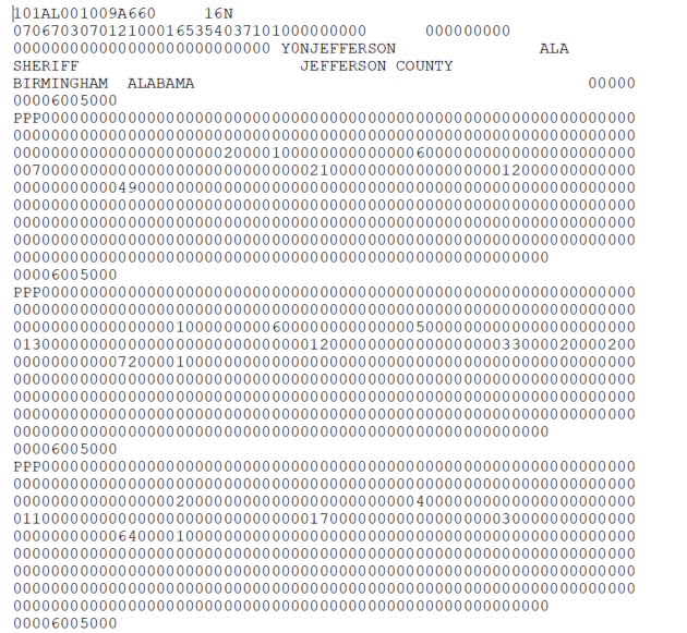
Figure 2.12: Fixed-width ASCII file for the 1960 Offenses Known and Clearances by Arrest data set.
The “fixed-width” part of the file type is how this works (the ASCII part basically means it’s a text file). Each row is the same width - literally the same number of characters, including blank spaces. So you must tell the software you are using to process this file - by literally writing code in something called a “setup file” but is basically just instructions for whatever software you use (R, SPSS, Stata, SAS can all do this) - which characters are certain columns. For example, in this data the first character says which type of UCR data it is (1 means the Offenses Known and Clearances by Arrest data) and the next two characters (in the setup file written as 2-3 since it is characters 2 through 3 [inclusive]) are the state number (01 is the state code for Alabama). So we can read this row as the first column indicating it is an Offenses Known data, the second column indicating that it is for the state of Alabama, and so on for each of the remaining columns. To read in this data you’ll need a setup file that covers every column in the data (some software, like R, can handle just reading in the specific columns you want and don’t need to include every column in the setup file).
The second important thing to know about reading in a fixed-width ASCII file is something called a “value label.”22 For example, in the above image we saw the characters 2-3 is the state and in the row we have the value “01” which means that the state is “Alabama.” Since this type of data is trying to be as small as efficient as possible, it often replaces longer values with shorter one and provides a translation for the software to use to convert it to the proper value when reading it. “Alabama” is more characters than “01” so it saves space to say “01” and just replace that with “Alabama” later on. So “01” would be the “value” and “Alabama” would be the “label” that it changes to once read.
Fixed-width ASCII files may seem awful to you reading it today, and it is awful to use. But it appears to be an efficient way to store data back many decades ago when data releases began but now is extremely inefficient - in terms of speed, file size, ease of use - compared to modern software so I’m not sure why they still release data in this format. But they do, and even the more modern (if starting in 1991, before I was born, is modern!) NIBRS data comes in this format. For you, however, the important part to understand is not how exactly to read this type of data, but to understand that people who made this data publicly available (such as myself and the team at NACJD) must make this conversion process.23 This conversion process, from fixed-width ASCII to a useful format is the most dangerous step taken in using this data - and one that is nearly entirely unseen by researchers.
Every line of code you write (or, for SPSS users, click you make) invites the possibility of making a mistake.24 The FBI does not provide a setup file with the fixed-width ASCII data so to read in this data you need to make it yourself. Since some UCR data are massive, this involves assigning the column width for thousands of columns and the value labels for hundreds of different value labels.25 A typo anywhere could have potentially far-reaching consequences, so this is a crucial weak point in the data cleaning process - and one in which I have not seen anything written about before. While I have been diligent in checking the setup files and my code to seek out any issues - and I know that NACJD has a robust checking process for their own work - that doesn’t mean our work is perfect.26 Even with perfection in processing the raw data to useful files, decisions we make (e.g. what level to aggregate to, what is an outlier) can affect both what type of questions you can ask when using this data, and how well you can answer them.
References
Arson is also an index crime but was added after these initial seven were chosen and is not included in the crimes data set (though is available separately) so is generally not included in studies that use index crimes.↩︎
There is also a human trafficking data set though this is a newer data set and rarely used so I will not cover it in this book.↩︎
Index crimes are sometimes capitalized as “Index Crimes” though I’ve seen it written both ways. In this book I keep it lowercase as “index crimes.”↩︎
I’ve also seen the justification that aggravated assault is more serious since it uses a weapon, though as the UCR subcategory of aggravated assault without a weapon clearly shows, aggravated assault does not require use of a weapon.↩︎
Simple assault is first available in 1964. Index crime data is available since 1960.↩︎
The FBI’s report for arrests does include simple assault so the second reason people may not include it does not apply here.↩︎
UCR data provides no information about the harm caused to victims. The new FBI data set NIBRS actually does have a variable that includes harm to the victim so if you’re interested in measuring harm (an understudied topic in criminology), that is the data set to use.↩︎
From 1960-2022, there were 39 agency-years with a negative count of murders.↩︎
Jurisdiction here refers to the boundaries of the local government, not any legal authority for where the officer can make arrests. For example, the Los Angeles Police Department’s jurisdiction in this case refers to crimes that happen inside the city or are otherwise investigated by the LAPD - and are not primarily investigated by another agency.↩︎
Some states do mandate that their agencies report, but this is not always followed.↩︎
This data is also sometimes called the “Police Employees” data set.↩︎
If you’re familiar with the National Incident-Based Reporting System (NIBRS) data that is replacing UCR, this data set is the closest UCR data to it, though it is still less detailed than NIBRS data.↩︎
The first year where transgender as a group was a considered a bias motivation was in 2013.↩︎
It also includes the value of items stolen during rapes and murders, if anything was stolen.↩︎
I will refer to this an “ORI”, “ORI code”, and “ORI number”, all of which mean the same thing.↩︎
In the NIBRS data (another FBI data set) the ORI uses a 9-digit code - expanding the 5 numbers to 7 numbers.↩︎
For most fixed-width ASCII files there are also missing values where it’ll have placeholder value such as -8 and the setup file will instruct the software to convert that to NA. UCR data, however, does not have this and does not indicate when values are missing in this manner.↩︎
For those interested in reading in this type of data, please see my R package asciiSetupReader.↩︎
Even highly experienced programmers who are doing something like can make mistakes. For example, if you type out “2+2” 100 times - something extremely simple that anyone can do - how often will you mistype a character and get a wrong result? I’d guess that at least once you’d make a mistake.↩︎
With the exception of the arrest data and some value label changes in hate crimes and homicide data, the setup files remain consistent so a single file will work for all years for a given data set. You do not need to make a setup file for each year.↩︎
For evidence of this, please see any of the openICPSR pages for my detail as they detail changes I’ve made in the data such as decisions on what level to aggregate to and mistakes that I made and later found and fixed.↩︎